НОУ ИНТУИТ | Практикум по компьютерной геометрии. Лекция 1: Первое знакомство с пакетом Mathematica

Учитесь и получайте официальные документы БЕСПЛАТНО. Вы можете поддержать наш проект.

Регистрация Вход

Твой путь к знаниям!

Опубликован: 27.12.2010 | Уровень: специалист | Доступ: платный

|

Вам нравится? Нравится 14 студентам

| Поделиться |

Поддержать программу

(4.22) Найти параметрические уравнения кривых, зная их натуральные уравнения (здесь R = 1/k ): a) R = as .

Решение 1. Имеем

$\text{In[244]:=} k[s\_]\; :=\; \frac{1}{as}; \\ \\ \text{In[245]:=} \alpha [s\_]=\int k[s]ds}\\ \\ \text{Out[245]=} \frac{\text{Log}[s]}{a}\\ \\ \text{In[246]:=} x[s\_]=\int\text{Cos}[\alpha [s]] ds\\ \phantom{\text{In[246]:=}} y[s\_]=\int\text{Sin}[\alpha [s]] ds}\\ \\ \text{Out[246]=} \frac{as\left(a\text{Cos}\left[\frac{\text{Log} [s]}{a}\right] + \text{Sin} \left[\frac{\text{Log}[s]}{a}\right]\right)}{1+a^2}\\ \\ \text{Out[247]=} \frac{as\left(-\text{Cos}\left[\frac{\text{Log}[s]}{a}\right]+a \text{Sin} \left[\frac{\text{Log}[s]}{a}\right]\right)}{1+a^2}\\ \\ \text{In[248]:=} \{x[s],\; y[s]\} \\ \\ \text{Out[248]=} \left\{\frac{as\left(a\text{Cos}\left[\frac{\text{Log}[s]}{a}\right]+\text{Sin}\left[\frac{\text{Log}[s]}{a}\right]\right)}{1+a^2}, \; \frac{as\left(-\text{Cos}\left[\frac{\text{Log}[s]}{a}\right]+a\text{Sin}\left[\frac{\text{Log}[s]}{a}\right]\right)}{1+a^2}\right\}$

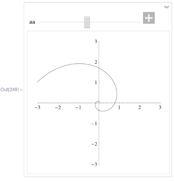
Изобразим полученные кривые для параметра в пределах от 0.1 до 20 и изучим их зависимость от параметра , изменяющегося в пределах от 0.05 до 1 с начальным значением 0.5:

$\text{In[249]:=} \\ \phantom{\text{In}}\text{Module}[\{x,y,a\}, \\ \phantom{\text{InM}}x[s\_]:=\frac{as\left(a \text{Cos} \left[ frac{\text{Log}[s]}{a}\right] + \text{Sin}\left[\frac{\text{Log}[s]}{a}\right]\right)}{1+a^2};\\ \phantom{\text{InM}}y[s\_]:=\frac{as\left(-\text{Cos}\left[\frac{\text{Log}[s]}{a}\right]+a \text{Sin}\left[\frac{\text{Log}[s]}{a}\right]\right)}{1+a^2}; \\ \phantom{\text{InM}}\text{Manipulate}[\text{ParametricPlot}[\{x[s], y[s]\}\text{ /. } a\to aa, \\ \phantom{\text{InMMa}}\{s,0.1,20\},\text{PlotRange} \to \{\{-3, 3\}, \{-3,3\}\}, \text{ImageSize}\to 250], \\ \phantom{\text{InMM}}\{\{aa, 0.5\}, 0.05,1\}] \\ \phantom{\text{In}}]$

$\text{In[250]:=Clear}[k, \alpha, x,y]\}$

Решение 2. Вместо явного интегрирования решим систему дифференциальных уравнений:

$\text{In[251]:=} \\ \phantom{\text{In}}\text{res}=\text{DSolve}\left[\left\{\alpha'[s]==\frac{1}{as}, x'[s]==\text{Cos}[\alpha [s]], y'[s]==\text{Sin}[\alpha [s]]\right\}\right., \\ \phantom{\text{In[251]}}\left.\{\alpha [s], x[s], y[s]\}, s\right] \\ \\ \text{Out[251]=}\{\{\alpha [s] \to C[1]+\frac{\text{Log}[s]}{a},\\ \phantom{\text{Out[251]=}\{\{}x[s] \to C[2]+\frac{as\left(a \text{Cos}\left[C[1] + \frac{Log[s]}{a}\right]+\text{Sin}[C[1]+\frac{\text{Log}[s]}{a}]\right)}{1+a^2},\\ \phantom{\text{Out[251]=}\{\{}y[s] \to C[3]+\frac{as\left(-\text{Cos}\left[C[1]+\frac{\text{Log}[s]}{a}\right]+a \text{Sin}\left[C[1]+\frac{\text{Log}[s]}{a}\right]\right)}{1+a^2}\}\}$

Задав начальные значения констант равными нулю, получим (сравните с предыдущим результатом)

$\text{In[252]:=\{x[s], y[s]\} /. res[\![1]\!] /. \{C[1]}\to\text{0, C[2]} \to \text{0, C[3]} \to \text{0\} // Simplify} \\ \\ \text{Out[252]=}\left\{\frac{as\left(a \text{Cos}\left[\frac{\text{Log}[s]}{a}\right] + \text{Sin}\left[\frac{\text{Log}[s]}{a}\right]\right)}{1+a^2}, \frac{as\left(-\text{Cos}\left[\frac{\text{Log}[s]}{a}\right]+a \text{Sin} \left[\frac{\text{Log}[s]}{a}\right]\right)}{1+a^2}\right\}\\ \\ \text{In[253]:=Clear[k, } \alpha\text{, x, y, res]}$

Важное замечание. Численная реализация Решения 2 работает даже тогда, когда Mathematica не может посчитать интегралы. Проиллюстрируем это на примере:

$\tt In[254]:=k[s\_]=se^s;$

Первый способ:

$\tt In[255]:=$\alpha$[s\_]=$\int$k[s] ds \\ \\ Out[255]=$e^s$ (-1+s) \\ \\ In[256]:=x[s\_]=$\int$Cos[$\alpha$[s]] ds \\ \phantom{In[256]:=}y[s\_]=$\int$Sin[$\alpha$[s]] ds \\ \\ Out[256]=$\int$Cos[$e^s$(-1+s)] ds \\ \\ Out[257]=$\int$Sin[$e^s$(-1+s)] ds \\ \\ In[258]:=ParametricPlot[\{x[s], y[s]\}, \{s, 0.1, 1\}] \\ \\ Integrate::ilim : Invalid integration variable or limit(s) in 0.1'.>> \\ \\ Integrate::ilim : Invalid integration variable or limit(s) in 0.10001836734693878'.>> \\ \\ Integrate::ilim : Invalid integration variable or limit(s) in 0.10001836734693878'.>> \\ \\ \\ \phantom{In}General::stop : Further output of Integrate::ilib will be suppressed during this calculation.>>$

$\tt In[259]:=Clear[k, $\alpha$, x, y]$

Второй способ:

$\tt In[260]:= \\ \\ \phantom{In}k[s\_]:=s$e^s$; \\ \phantom{In}res= \\ \phantom{Inr}NDSolve[\{$\alpha$'[s]==k[s], x'[s]==Cos[$\alpha$[s]], y'[s]==Sin[$\alpha$[s]], \\ \phantom{InrND}$\alpha$[0]==0, x[0]==0, y[0]==0\}, \{$\alpha$[s], x[s], y[s]\}, \{s,0,1\}]\} \\ \\ Out[261]=\{\{$\alpha$[s]$\to$InterpolatingFunction[\{\{0., 1.\}\}, <>][s], \\ \phantom{Out[261]=\{\{}x[s]$\to$InterpolatingFunction[\{\{0., 1.\}\}, <>][s], \\ \phantom{Out[261]=\{\{}y[s]$\to$InterpolatingFunction[\{\{0., 1.\}\}, <>][s]\}\} \\ \\ In[262]:=$\gamma$[s\_]=\{x[s], y[s]\} /. res[\![1]\!] // Simplify \\ \\ Out[262]=\{InterpolatingFunction[\{\{0., 1.\}\}<>][s], \\ \phantom{Out[262]=\{}InterpolatingFunction[\{\{0., 1.\}\},<>][s]\} \\ \\ In[263]:=ParametricPlot[$\gamma$[s], \{s, 0, 1\}]$

$\tt In[264]:=Clear[k, $\gamma$]$

Построить пространственную кривую с кривизной k[t] = 1 + sin[t]^2 и кручением и[t] = cos[t] .

$\tt In[265]:=\\ \\ \phantom{In}k[t\_]=1+Sin$[t]^2$; k[t\_] = Cos[t]; $\gamma$[t\_] := \{x[t], y[t], z[t]\}; \\ \phantom{In}eq[$\xi$\_, $\eta$\_]:=Table[$\xi$[\![i]\!]==$\eta$[\![i]\!], \{i,3\}]; \\ \phantom{In}v[t\_]=\{v1[t], v2[t], v3[t]\}; \\ \phantom{In}n[t\_]=\{n1[t], n2[t], n3[t]\}; \\ \phantom{In}b[t\_]=\{b1[t], b2[t], b3[t]\};\\ \\ In[269]:= \phantom{In}frenet=eq[$\gamma$'[t], v[t]]$\sim$Join$\sim$eq[v'[t], k[t]n[t]]$\sim$Join$\sim$ \\ \phantom{Infr}eq[n'[t], -k[t]v[t] + $\kappa$[t]b[t]]$\sim$Join$\sim$ eq[b'[t], -$\kappa$[t]n[t]] \\ \\$

$\tt Out[269]=\{x'[t] == v1[t], y'[t] == v2[t], \\ \phantom{Out[269]=\{}z'[t] == v3[t], v1'[t] == n1[t] (1+Sin[t]^{2}), \\ \tt \phantom{Out[269]=}v2'[t] == n2[t] (1+Sin[t]^{2}), v3'[t] == n3[t] (1+Sin[t]^{2}), \\ \phantom{Out[269]=}n1'[t] == b1[t] Cos[t] + (-1-Sin[t]^{2}) v1[t], \\ \phantom{Out[269]=}n2'[t] == b2[t] Cos[t] + (-1-Sin[t]^{2}) v2[t], \\ \phantom{Out[269]=}n3'[t] == b3[t] Cos[t] + (-1-Sin[t]^{2}) v3[t], \\ \phantom{Out[269]=}b1'[t] == -Cos[t] n1[t], \\ \phantom{Out[269]=}b2'[t] == -Cos[t] n2[t], b3'[t] == -Cos[t] n3[t]\}$

$\tt In[270]:= \\ \\ \phantom{In}res=NDSolve[frenet$\sim$Join$\sim$eq[$\gamma$[0], \{0,0,0\}]$\sim$Join$\sim$ \\ \phantom{Inres}eq[v[0], \{1,0,0\}] $\sim$Join$\sim$eq[n[0], \{0,1,0\}$\sim$Join$\sim$ \phantom{Inres}eq[b[0], \{0,0,1\}], $\gamma$[t]$\sim$Join$\sim$v[t]$\sim$Join$\sim$n[t]$\sim$Join$\sim$b[t], \\ \phantom{Inre}\{t,0,100\}]$

$\tt Out[270]=\{\{x[t]$\to$InterpolatingFunction[\{\{0., 100.\}\}, <>][t], \\ \phantom{Out[270]=\{\{}y[t]$\to$InterpolatingFunction[\{\{0., 100.\}\}, <>][t], \\ \phantom{Out[270]=\{\{}z[t]$\to$InterpolatingFunction[\{\{0., 100.\}\}, <>][t], \\ \phantom{Out[270]=\{\{}v1[t]$\to$InterpolatingFunction[\{\{0., 100.\}\}, <>][t], \\ \phantom{Out[270]=\{\{}v2[t]$\to$InterpolatingFunction[\{\{0., 100.\}\}, <>][t], \\ \phantom{Out[270]=\{\{}v3[t]$\to$InterpolatingFunction[\{\{0., 100.\}\}, <>][t], \\ \phantom{Out[270]=\{\{}n1[t]$\to$InterpolatingFunction[\{\{0., 100.\}\}, <>][t], \\ \phantom{Out[270]=\{\{}n2[t]$\to$InterpolatingFunction[\{\{0., 100.\}\}, <>][t], \\ \phantom{Out[270]=\{\{}n3[t]$\to$InterpolatingFunction[\{\{0., 100.\}\}, <>][t], \\ \phantom{Out[270]=\{\{}b1[t]$\to$InterpolatingFunction[\{\{0., 100.\}\}, <>][t], \\ \phantom{Out[270]=\{\{}b2[t]$\to$InterpolatingFunction[\{\{0., 100.\}\}, <>][t], \\ \phantom{Out[270]=\{\{}b3[t]$\to$InterpolatingFunction[\{\{0., 100.\}\}, <>][t]\}\}$

$\tt In[271]:= \\ \phantom{In[271]:=}Manipulate[ParametricPlot3D[$\gamma$[t] /. Res[\![1]\!], \{t,0,aa\}, \\ \phantom{In[271]:=Ma}PlotRange$\to$\{\{-1,1\}, \{0,2\}, \{-1,1\}\}, \\ \phantom{In[271]:=Ma}PlotPoints$\to$Round[$\frac{10}{11}$aa+$\frac{100}{11}$], ImageSize$\to$250], \\ \phantom{In[271]:=M}\{\{aa, 44\}, 1, 100\}]$

Дальше >>

Практикум по компьютерной геометрии

Практикум по компьютерной геометрии

Первое знакомство с пакетом Mathematica

Вопросы и ответы

Студенты

Авторизоваться

Практикум по компьютерной геометрии

Практикум по компьютерной геометрии

Первое знакомство с пакетом Mathematica

Вопросы и ответы

Студенты